DISCOVER

A recurrent controller writes expression trees token by token and is trained on its own best-rewarded draws; the coefficients come from a platform refit.

algorithm

discover

score

reward max

cost

heavy

derivatives

finite_diff autograd

equation form

EVOLUTION REGRESSION

data layout

grid tabular

Usage

import kd
from kd import DiscoverConfig

dataset = kd.load_chafee_infante()
model = kd.Model(
    algorithm="discover",
    generations=200,
    config=DiscoverConfig.chafee_preset(seed=42),
)
model.fit(dataset)

Main parameters

Parameter	Default	Resume	Description
batch_size	16	resume-safe	Controller samples per Runner iteration.
learning_rate	0.001	resume-safe	Controller learning rate.
entropy_weight	0.005	resume-safe	Exploration-entropy weight.
reward_alpha	0.01	resume-safe	Reward sparsity trade-off.
max_length	15	resume-safe	Maximum generated expression length.
epsilon	0.1	resume-safe	Risk-seeking reward quantile: the top-epsilon fraction of a batch's rewards feeds the policy-gradient update.
magnitude_filter	False	resume-safe	Reject fitted coefficients outside the reference magnitude bounds.

All fields of DiscoverConfig

Field	Type	Default
n_iterations	int	2000
seed	int	0
library	LibraryConfig	LibraryConfig(...)
min_length	int	2
max_length	int	15
batch_size	int	16
num_units	int	16
num_layers	int	1
embedding_dim	int	4
observe_parent	bool	True
observe_sibling	bool	True
observe_action	bool	False
observe_dangling	bool	False
use_embedding	bool	False
attention	bool	False
attn_length	int	10
initializer	Literal['xavier', 'zeros']	xavier
epsilon	float	0.1
baseline	str	R_e
entropy_weight	float	0.005
gamma	float	0.5
reward_alpha	float	0.01
learning_rate	float	0.001
entropy_gamma	float	1.0
max_diff_order	int \| None	4
use_repeat_prior	bool	True
repeat_tokens	list[str]	['add']
repeat_max	int	5
use_trig_prior	bool	True
use_inverse_prior	bool	True
use_diff_descendant_prior	bool	True
use_diff_child_prior	bool	True
soft_length_loc	float \| None	None
soft_length_scale	float	5.0
stability_selection	int	0
stability_queue_capacity	int	10
magnitude_filter	bool	False
diagnostic_scaffold	bool	False
diagnostic_scaffold_diffusion_tokens	tuple[str, ...]	()
diagnostic_scaffold_reaction_tokens	tuple[str, ...]	()
diagnostic_scaffold_root_tokens	tuple[str, ...]	('add', 'sub')
diagnostic_scaffold_neutral_tokens	tuple[str, ...]	()
token_bias_tokens	tuple[str, ...]	()
token_bias_weight	float	0.0
pinn	PINNConfig \| None	None

Search space

DISCOVER samples expression trees from operator and variable tokens, without a fixed candidate-term library. In the standard PDE vocabulary, products, quotients and trigonometric expressions can use u, x and t, with spatial derivatives represented by diff_x(u) and diff2_x(u). Repeated multiplication forms powers. Priors restrict nesting of derivatives and trigonometric functions. Coordinate tokens permit coordinate-dependent fits.

The facade's grid vocabulary is fixed to u, x, t, diff_x, diff2_x. Other field names, extra fields and extra spatial axes are refused. An additional dataset axis does not add tokens automatically. The standard vocabulary contains no mixed derivative or third-order derivative token. max_diff_order can further restrict the vocabulary but cannot add an absent token or override another structural prior. The facade controls iteration count with generations; n_iterations does not set its loop length. Without pinn, the PDE path evaluates derivatives from the observed grid by finite differences and requires no pretrained weights or optional backend. With pinn set, the same vocabulary is searched in PINN mode, where a neural network is trained on the data and derivatives are taken from the network by automatic differentiation.

Tabular regression

Tabular mode is selected by the input data, without a mode parameter. Its vocabulary is derived from the feature columns plus add, sub, mul, div, sin, cos, exp, log and a fitted const terminal. No derivative tokens or configured term library are used. Each distinct candidate's constants are fitted before scoring. The recurrent controller and training rule remain the same, while complexity counts tokens instead of additive terms.

Method

An LSTM samples token sequences in pre-order, conditioned on the parent and left sibling of each slot. Structural priors mask illegal choices: expression length and token-repetition bounds, addition or subtraction below a derivative, derivative arguments other than fields or permitted derivative expressions, unary operators directly below their inverse, and excessive cumulative derivative order. The standard priors also prevent nested derivatives and trigonometric nesting. Sequences that fail length or legality checks are dropped and surviving expressions are deduplicated before scoring.

In PDE mode the platform splits top-level additions into terms, fits their coefficients by dense least squares against the time derivative, and computes NMSE. Subtraction is carried by signed terms. In tabular mode, all-constant candidates are rejected; unique traversals fit constants with a scale-free BFGS objective before serialization as numeric literals. The platform then scores the whole expression as one regression term with a fitted outer scale.

Risk-seeking policy gradient retains the top epsilon fraction of valid rewards, subtracts a scalar baseline, and takes an Adam step on the policy loss plus an entropy bonus. Invalid fits receive zero reward and are excluded from training. The champion changes only on strict improvement, so ties retain the incumbent. The seed controls both initial network weights and token sampling. One controller iteration is one KD iteration, controlled by generations.

PINN mode

Setting pinn on grid data selects PINN mode. On a fresh call, a fully connected network is first pretrained on the observations: every grid point, or the share given by obs_ratio. A resumed call loads the stored network without pretraining. Candidates are then scored on collocation points sampled inside the data domain, with the time derivative on the left-hand side and every spatial derivative taken from the network by automatic differentiation.

After n_iterations generations, and then after every cycle_n_iterations generations, the network is retrained on the data loss plus coef_pde times the residual of the best equation found so far, and the search continues on the derivatives of the retrained network. The champion is re-scored on each new network before the search resumes. On a fresh call, generations is the total number of search generations, so a retraining phase runs only when n_iterations is smaller than generations. On resume, the phase boundaries use the generation count over all segments of the run; the resumed call's generations add to that count. A phase on a call's last generation is not run in that call. If the earlier segment ended on such a boundary, the resumed call runs that phase first, before its first generation. When stability_selection is positive, the final equation is chosen among the top candidates of the last cycle by refitting each on bootstrap resamples.

The time of the pretraining and of each retraining phase grows with the number of epochs times the number of training points. The library defaults of pretrain_epoch, pinn_epoch and n_collocation are the research budget of the reference configuration.

Result interpretation

The reward combines fit and complexity as (1 - reward_alpha * complexity) / (1 + sqrt(nmse)), clipped to [0, 1]. Complexity is the term count for PDEs and token count for tables. NMSE alone does not rank expressions. A surviving coordinate term indicates dependence on that coordinate and should be interpreted according to the physical model being sought.

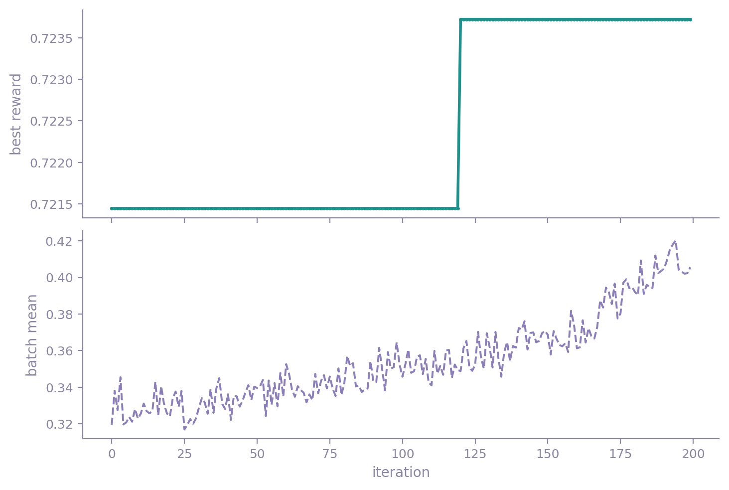
For PDEs, model.best_expr_ is the sampled structure and model.result_.equation carries the coefficients from the same least-squares fit used in scoring. The recorder's best_reward is non-decreasing; n_eval_valid distinguishes invalid sampling from valid candidates with poor fits. An improving champion at the final iteration suggests additional search may still change the result; a flat curve alone does not identify the cause.

In PINN mode the final equation is fitted on the collocation points, so the target and the residuals of the result have one entry per collocation point, and the result config records provider_kind as autograd. On a fresh call, the recorder carries the pretraining outcome in the pinn_pretrain_* series; a resumed segment's recorder has no such series. Each segment records one entry per retraining phase it executes in pinn_cycle_idx, pinn_phase_ran, pinn_data_loss, pinn_physics_loss, pinn_total_loss, pinn_epochs_run and pinn_train_seconds. A phase with no valid best equation is recorded with pinn_phase_ran equal to 0 and leaves the network unchanged.

Tabular results carry a REGRESSION equation with the target column on the left. The expression retains its fitted numeric literals and one outer least-squares scale. model.result_.pareto_front() exposes nondominated expressions with their token counts, loss and outer scale; the corresponding series are pareto_expressions, pareto_complexity, pareto_loss and pareto_scale. The inner constants and outer scale are distinct fitted values.

Python setup

A kd.TabularDataset selects tabular mode in Model.fit(). A typed DiscoverConfig can supply a different library, which is Python-only and unavailable through JSON params. pinn takes a PINNConfig, exported from kd.search, or a JSON object of its fields, in which every omitted key keeps its default. DiscoverConfig.burgers_preset(pinn=PINNConfig(...)) combines a reference preset with PINN mode through config=. A sketch, an EarlyStoppingCallback and a kd.TabularDataset are refused together with pinn.

References

Du et al. (2024). "DISCOVER: Deep identification of symbolically concise open-form partial differential equations via enhanced reinforcement learning". Phys. Rev. Research 6, 013182. Paper · arXiv:2210.02181

Code: menggedu/DISCOVER

Implementation notes. KD implements the reinforcement-learning search, structural priors, PINN mode and its optional stability selection. The paper's genetic operators and dynamic subtree bank are not implemented. Risk-seeking policy gradient is the training strategy; PQT has zero weight in the reference's shipped configuration, and PPO is not implemented. The configured quantile follows DSO-PyTorch, while the paper used 0.02. Unary diff_x(u) replaces the paper's binary diff(u, x) for one-dimensional spatial differentiation.

Dense least squares and the stability-selection statistic std / mean follow the reference code; the paper prints the reciprocal statistic. The optional coefficient-magnitude rejection is disabled unless configured. A follow-up method trains a neural surrogate and differentiates it by autograd; KD runs it as PINN mode. The retraining phases are placed inside the generations loop by n_iterations and cycle_n_iterations, and the reference's cycle count n_cycles is read only by the standalone cycle runner.

Worked example

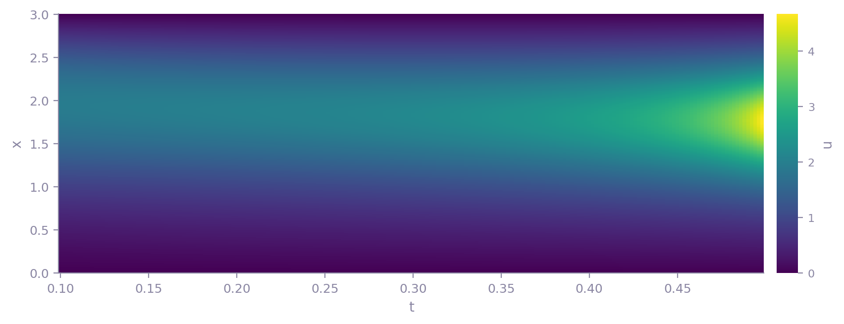
The run below uses the Chafee-Infante dataset that ships with KD: a 301 × 200 grid over x in [0, 3] and t in [0.1, 0.5], carrying a single hump held at zero at both ends of the interval. Above u = 1 the cubic term is larger than the linear one, so the hump climbs from 1.94 at the first time step to 4.67 at the last while diffusion keeps its profile smooth.

The observed field over its physical spatial and time coordinates.

The equation returned by the run:

	Equation
Discovered	\(u_{t} = 0.9808 t^{3} u + 0.9808 u^{3} - 0.9946 u + 0.9754 u_{xx}\)
Reference	\(u_t = u_{xx} -u +u^3\)

The returned expression contains the reference diffusion and reaction terms, plus a time-dependent cubic contribution. The displayed coefficients are fitted on this run. The search receives operator tokens (add, mul, div, diff_x, diff2_x, diff3_x, n2, n3) and composes the candidate expressions.

The fitted derivative target, its equation prediction, and predicted minus measured values. The first two panels share a color scale; the residual has its own scale, with any clipping disclosed on the figure.

Example diagnostics

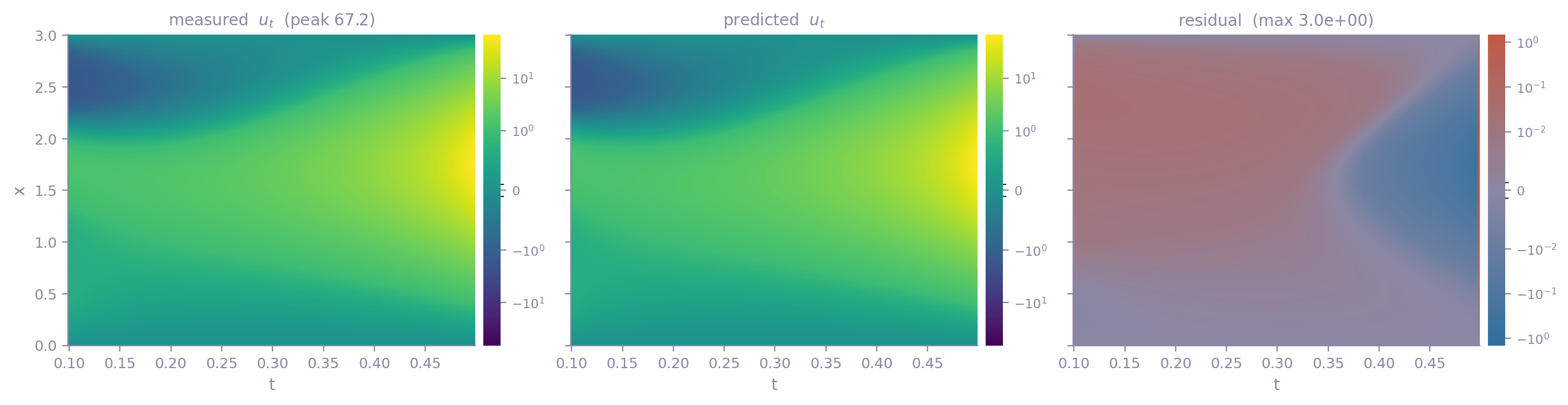
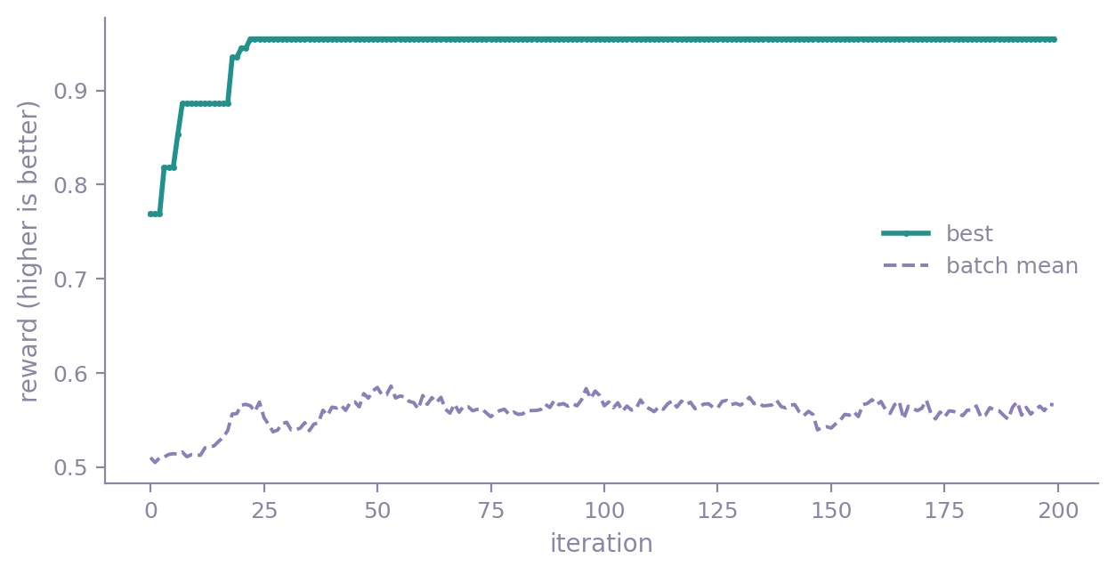
This run has reward 0.955317 and NMSE 0.0002362.

The reward divides a term-count penalty by one plus the square root of NMSE. Every derivative in this run is a finite difference of the observations.

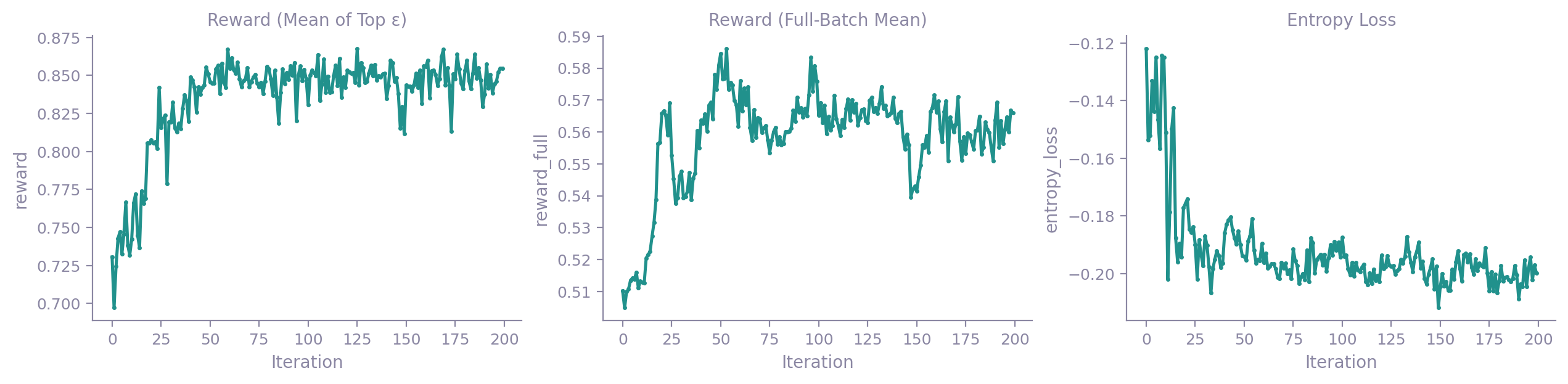
The search is recorded as well. kd.VizEngine renders the per-iteration record; alongside the universal convergence curve, DISCOVER contributes four diagnostic panels of its own, three of which this run drew (the full list is under Visualization):

The best native score is shown above the algorithm's population diagnostic, when one is recorded. Each panel retains its own score scale.

The algorithm's diagnostic panels, using the same data and plot functions as the full report.

viz = kd.VizEngine(output_dir="out/chafee-infante")
viz.render_all(model.result_, algorithm=model.algorithm_, dataset=dataset)

Tabular example

config = DiscoverConfig(
    seed=0, batch_size=1000, max_length=15, reward_alpha=0.005
)
model = kd.Model(algorithm="discover", generations=200, config=config)
model.fit(kd.load_tlc_cc())

The table layout is described under data requirements.

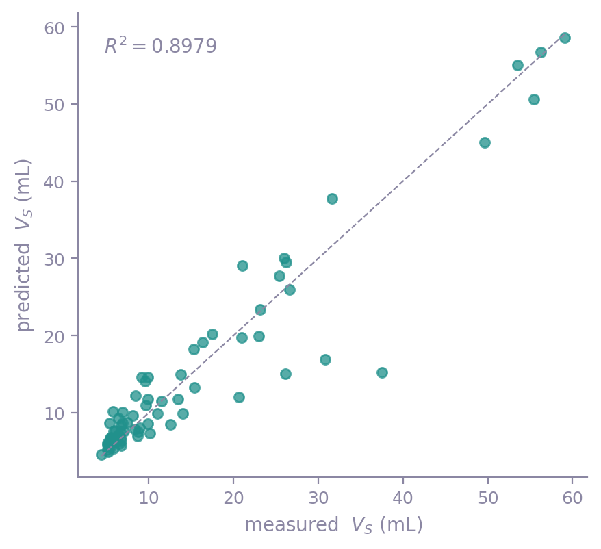
The run below uses that table. Its 74 rows come from an automated column-chromatography platform: the features are the thin-layer retardation factor R_F and the petroleum-ether fraction r of the eluent, and the target is the retention volume V_S in millilitres. A formula relating the three has been published for this table (Xu et al., 2025). The settings are seed 0, 200 iterations, 1000 draws per iteration, expressions of at most 15 tokens, and reward_alpha 0.005.

	Equation
Discovered	\(V_S = \dfrac{r}{0.1507\,R_F + 0.0111}\)
Reference	\(V_S = \dfrac{r}{0.147\,R_F + 0.0114}\)

Both rows are written as r / (a R_F + b). Scoring is scale-free, so the search returns a bare expression with the outer coefficient fitted beside it, and this answer arrived as 6.634 times r / (R_F + 0.0737); dividing through puts it in the published form. The two coefficients land 2.5% and 2.6% from the published pair, from one run at a fixed seed, with the search given four arithmetic operators and two column names rather than any candidate terms.

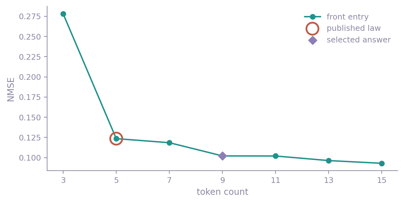
That expression is five tokens long, and it is an entry on the run's Pareto front rather than the answer the run selected. Three of the 74 rows were measured at r = 0, where the formula returns zero against measured volumes of 4.41, 5.17 and 5.86 mL. The selected expression returns nonzero volumes at r = 0 and fits the table more closely: nine tokens, at an nmse of 0.1021 against the five-token law's 0.1235.

The final Pareto table lists complexity, loss, outer scale and mathematical expression for each candidate. Compare the five-token law with the selected nine-token expression using the values in the table.

Predicted values against the measured target, with the diagonal denoting exact agreement and R² computed over the full fit.

The best native score is shown above the algorithm's population diagnostic, when one is recorded. Each panel retains its own score scale.

Full report

The PDE run's returned equation includes an explicit time term. The current forward integrator does not support that term, so the field-reconstruction panels are unavailable. The derivative-fit comparison and search diagnostics above do not require forward integration.

Full HTML report from the same run, with all figures, captions and raw result data.

The tabular run has its own report:

Full HTML report from the same run, with all figures, captions and raw result data.