Breaking waves
EqGPT discovered a law for breaking-wave surface elevation from 12 wave-tank
experiments (Xu et al., Nat Commun 16, 10255,
2025). KD hosts EqGPT as a search
plugin and reproduces that published result, with permission of the authors, on
the same scattered (t, x, eta) measurements:
In KD's notation the surface elevation is the field u, so the recovered
right-hand side is the term set {u_x, u_xxx, diff2_x(mul(u, u_x))} with
per-experiment coefficients.
import kd
from kd.core.expr import to_sympy
from kd.data.loaders import load_wave_breaking_datasets
Optional data preview
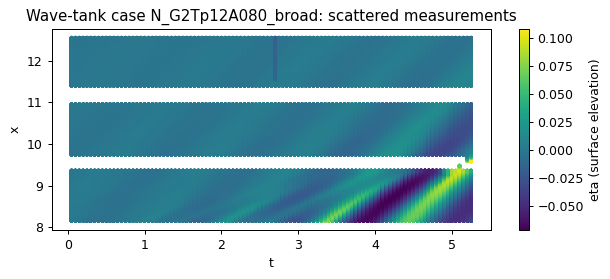
WaveBreaking.pkl holds surface-elevation records from the BUBER and EURUS
campaigns in the 27.2 m glass-walled wave tank at Imperial College London,
where the air-water interface was reconstructed frame by frame from three
cameras running at 20 Hz; the paper's discovery uses the 12 "N" experiments. Each case is a scattered
point cloud (t, x, eta) with no grid, so the dataset is SCATTERED topology.
EqGPT fits all 12 cases; the preview below shows the first N case in sorted
order. kd.preview describes its axes and field, and kd.viz.plots.plot_field
draws the observed surface elevation. These preview calls are optional and do
not affect the fit. The later report describes the fitted equation and its
diagnostics.
cases = load_wave_breaking_datasets(case_filter="N")
primary_name = next(iter(cases))
primary_ds = cases[primary_name]

print(f"N cases ({len(cases)}): {', '.join(cases)}")
kd.preview(primary_ds)
kd.viz.plots.plot_field(primary_ds)
N cases (12): N_G2Tp12A080_broad, N_G2Tp12A090_broad, N_G2Tp12A100_broad, N_G2Tp12A105_broad, N_G2Tp13A090_broad, N_G2Tp13A096_broad, N_G2Tp13A105_broad, N_G2Tp13A130_broad, N_G3Tp12A083_broad, N_G3Tp12A095_broad, N_G3Tp12A100_broad, N_G3Tp12A117_broad
Dataset: wave-breaking-N_G2Tp12A080_broad
Axes:
     t | n=507868 | range [0.050, 5.250] | step n/a (scattered)
     x | n=507868 | range [8.148, 12.548] | step n/a (scattered)
Fields:
     u | dtype=float64 | shape=(507868,) | min=-0.071 max=0.109 mean=-0.000 (NaN=0)
LHS: u_t  (field='u', axis='t')
Status: ready to fit
Multi-case fit
EqGPTConfig.wave_preset pins the paper's setup: multi-case wave mode
(case_filter="N"), sparsity_alpha=0.02. Per generation the pretrained GPT
proposes candidate right-hand sides; KD scores each candidate on every
experiment (per-case surrogate and least-squares fit) and keeps the candidate
with the best mean reward over the cases that scored successfully. seed=21
makes the run reproduce the same result each time, through KD's CPU torch RNG
stream.
The cell below runs a 5-generation search across all 12 experiments, loading the per-case surrogates and the measurement records.
DEMO_SEED = 21

model = kd.Model(
    algorithm="eqgpt",
    generations=5,
    config=kd.EqGPTConfig.wave_preset(seed=DEMO_SEED, primary_case=primary_name),
).fit(primary_ds)

print(f"Reproduced structure : {to_sympy(model.best_expr_)}")
print(f"Best mean reward     : {model.best_score_:.4f}")
[kd] Generation   1/5 | best EqGPT reward=0.9486 | expr=u_x + u_xxx + (u*u_x)_xx


[kd] Generation   2/5 | best EqGPT reward=0.9486 | expr=u_x + u_xxx + (u*u_x)_xx


[kd] Generation   3/5 | best EqGPT reward=0.9486 | expr=u_x + u_xxx + (u*u_x)_xx


[kd] Generation   4/5 | best EqGPT reward=0.9486 | expr=u_x + u_xxx + (u*u_x)_xx


[kd] Generation   5/5 | best EqGPT reward=0.9486 | expr=u_x + u_xxx + (u*u_x)_xx


[kd] Done. Best: u_x + u_xxx + (u*u_x)_xx (EqGPT reward=0.9486)


Reproduced structure : u_x + u_xxx + (u*u_x)_xx
Best mean reward     : 0.9486
Recovered law vs the published equation
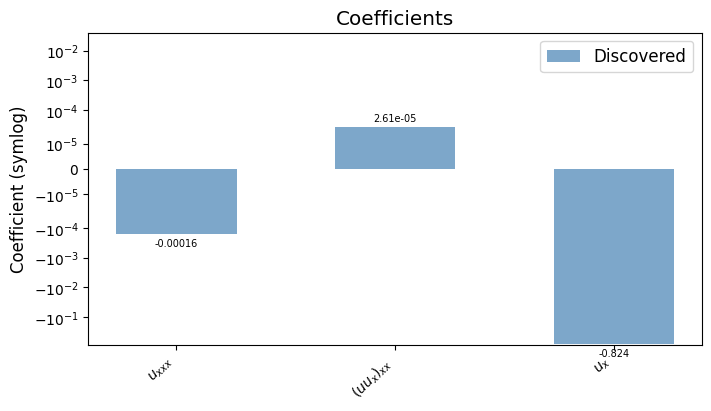
The published structure is eta_t = -c1*eta_x - c2*eta_xxx - c3*(eta*eta_x)_xx
(all three RHS terms). The fitted coefficients below are the primary case's
least-squares fit in the declared u_t = sum(c * term) domain; every
experiment gets its own coefficients (next section).
The coefficient panel shows their signs and magnitudes, with numeric labels when they span several orders of magnitude.
kd.viz.plots.plot_coefficient_bar(model.result_);
Render the report
model.report draws the figures this data supports and collects them into
one HTML page, displayed below. The page includes notes for figure families
that cannot be drawn; the same notes are available as report.warnings.
report = model.report("../out/wave_breaking")
report
Report: ../out/wave_breaking/report.html
Composable figure functions
Every figure in the report can also be drawn separately. The functions in
kd.viz.plots create a figure when called without ax; passing an existing
Matplotlib Axes lets you combine them in a larger layout. plot_plugin
uses the algorithm's own panel names and rendering method.
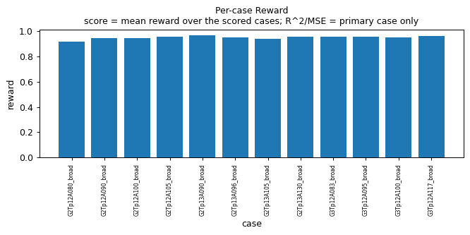
EqGPT's per-case reward panel has one bar per experiment, with the same discovered structure fitted separately to each case.
kd.viz.plots.plot_plugin(model.algorithm_, "per_case_reward");
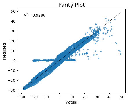
A platform figure works the same way. plot_parity puts the fitted
right-hand side against the measured u_t of the primary case, one point per
measurement.
kd.viz.plots.plot_parity(model.result_);
Reproduce this run
The run needs pretrained GPT weights, per-case surrogate checkpoints, and the measurement pickle. KD uses local assets when configured, and otherwise resolves the weights and surrogates from its Hub mirror (with permission of the authors). The measurement pickle must already be present.
| Asset | Location |
|---|---|
gpt_model/PDEGPT_wave_breaking.pt |
KD_EQGPT_ASSET_DIR, or the Hub cache |
model_save/wave_breaking/95_0_<case>(Non_unit)/Net_Sin_*.pkl |
KD_V1_WAVE_ASSETS, or the Hub cache |
WaveBreaking.pkl |
data/hf-knowledgediscover/ under the checkout root |
From examples/notebooks/:
uv run --with nbconvert python -m nbconvert --to notebook --execute --inplace wave_breaking.ipynb
To use local weight and surrogate trees, set KD_EQGPT_ASSET_DIR and
KD_V1_WAVE_ASSETS to their respective asset directories before running.
Next steps
examples/16_eqgpt.py-- EqGPT on synthetic Burgers data, no wave assets needed beyond the GPT weights.examples/09_compare_algorithms.py-- the same dataset scored by all seven algorithms against a single NMSE measure.examples/03_visualize.py-- the report pipeline on a fast synthetic fit, no assets at all.