Getting started: discover a PDE from field data
KD recovers the Burgers equation from a bundled benchmark dataset whose equation is known. This notebook loads the data, inspects the field, fits a symbolic model in one call, compares the result with the known equation, and plots the convergence curve.
import kd

ds = kd.load_burgers()
print(ds.ground_truth)
u_t = -u * u_x + 0.1 * u_xx
Look at the data
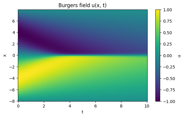
The dataset contains a field u sampled on an (x, t) grid. Before fitting, kd.preview prints the grid, the field, and the left-hand-side derivative that KD will use.
kd.preview(ds)
kd.viz.plots.plot_field(ds)
Dataset: burgers
Axes:
     x | n=256  | range [-8.000, 7.938] | step 0.0625 (uniform)
     t | n=201  | range [0.000, 10.000] | step 0.05 (uniform)
Fields:
     u | dtype=float64 | shape=(256, 201) | min=-1.000 max=1.000 mean=0.000 (NaN=0)
LHS: u_t  (field='u', axis='t')
Status: ready to fit
Fit a model
SGA-PDE searches over symbolic expression trees and scores candidate right-hand sides against the target derivative. generations sets the search budget. The value below is small enough to run quickly and large enough to recover a Burgers-like equation.
model = kd.Model(algorithm="sga", generations=5, seed=0, verbose=False).fit(ds)
print(model.result_.equation)
print(model.best_score_)
u_t = -u*u_x + 0.1002*u_xx
-28.776750720652373
Compare to ground truth
The discovered equation is KD's best symbolic right-hand side for u_t. The exact string can differ from the compact textbook form, so the check is whether it contains the nonlinear advection and diffusion terms.
print(f"Discovered  : {model.result_.equation}")
print(f"Ground truth: {ds.ground_truth}")
Discovered  : u_t = -u*u_x + 0.1002*u_xx
Ground truth: u_t = -u * u_x + 0.1 * u_xx
Visualize
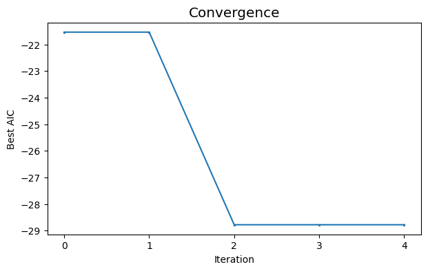
plot_convergence draws the recorded best-score curve, labels it with the
algorithm's score kind (AIC for SGA), and notes when the best score was reached
on the first iteration. It creates its own figure; the returned list contains
any plot notes.
from kd.viz.plots import plot_convergence

plot_convergence(model.result_);
The report
model.report writes every supported figure and an HTML report, and displays
the report here. The same files remain in the output directory.
model.report("../out/getting_started")
Report: ../out/getting_started/report.html
Next steps
This notebook used SGA-PDE. KD provides seven algorithms behind the same
kd.Model interface:
- Bring your own field data with
examples/02_your_data.py. - Compare all seven algorithms on one dataset against a single NMSE measure, with
examples/09_compare_algorithms.py: SGA, DLGA, DISCOVER, PySR, PySINDy, EqGPT, and LLM4ED. - Or run a single algorithm on its own: DISCOVER
(
07), DLGA (08), EqGPT (16), or LLM4ED (17).