SGA-PDE

A genetic search over expression trees; the coefficients come from the algorithm's own sparse regression.

algorithm

sga

score

AIC min

cost

medium

derivatives

finite_diff autograd

equation form

EVOLUTION

data layout

grid

Usage

import kd

dataset = kd.load_kdv()
model = kd.Model(algorithm="sga", generations=200, seed=42)
model.fit(dataset)
print(model.result_.equation)

Main parameters

Parameter	Default	Resume	Description
num	20	resume-safe	Population size.
p_cro	0.5	resume-safe	Crossover probability per generation.
p_mute	0.3	resume-safe	Per-node mutation probability.
p_var	0.5	resume-safe	Probability that a node in a freshly generated term tree is a variable rather than an operator.
p_rep	1.0	resume-safe	Replace-draw probability for non-elite members.
depth	4	resume-safe	Maximum term-tree depth.
width	5	resume-safe	Maximum terms per candidate equation.
aic_ratio	1.0	resume-safe	AIC complexity-penalty ratio.
lam	0.0	resume-safe	Internal STRidge ridge strength.

All fields of SGAConfig

Field	Type	Default
num	int	20
p_var	float	0.5
p_mute	float	0.3
p_cro	float	0.5
p_rep	float	1.0
seed	int	0
depth	int	4
width	int	5
aic_ratio	float	1.0
lam	float	0.0
d_tol	float	1.0
maxit	int	10
str_iters	int	10
normalize	int	2
dedup_mode	DedupMode	pre_prune
use_autograd	bool	False
field_model	FieldModel \| None	None
autograd_train_epochs	int	1000
autograd_train_lr	float	0.001
autograd_train_patience	int \| None	None
autograd_train_val_ratio	float	0.0
restart_interval	int \| None	None

Search space

SGA-PDE constructs an equation from expression trees over field values, spatial coordinates and derivatives. It fits coefficients during the search and needs no candidate-term library. A candidate has at most width searched trees plus the field itself, which is always included as a default column; the fitted law can therefore contain width + 1 terms. A law containing only that field is a valid outcome, while an empty law is excluded.

The left-hand-side axis is excluded from derivative denominators, precomputed terminals and coordinate leaves. The search space contains spatial derivatives and explicit spatial dependence. Mixed space-time derivatives, higher time derivatives and explicit time dependence require a different grammar. A term that still differentiates along the left-hand-side axis is discarded during execution. A derivative terminal that cannot be computed is removed from the run's vocabulary with a warning.

With autograd enabled, a field surrogate is trained before the search. It supplies the first-order derivative terminals; raw field leaves still come from the observations, and derivative operators inside trees still use SGA's finite differences. Surrogate training adds a separate cost before the first generation. SGA needs no optional package, pretrained weights or endpoint.

Method

A population contains candidate equations, each a set of up to width trees of depth at most depth. Leaves include every field, spatial coordinates and each field's first-order derivatives along every non-target axis. Only the left-hand-side field is prepended as the default regression column. Internal nodes are addition, subtraction, multiplication, division, square, cube and the first- and second-derivative operators. Tree roots exclude addition and subtraction because the term list already represents a sum.

Each generation applies crossover, evaluation and truncation, then mutation and replacement followed by another evaluation and truncation. Duplicate expressions are filtered by their expression keys. The evaluator executes each term into a column, removes non-finite and all-zero columns, prepends the field column, and fits coefficients with an internal STRidge tolerance sweep. An OLS baseline is followed by adaptive d_tol steps, bounded by maxit, with str_iters ridge iterations and column normalization of order 2. The fit's AIC ranks candidates for selection. One generation is one KD iteration, controlled by generations.

With restart_interval set to k, the population is re-drawn once k generations have been committed since the last draw. The re-draw happens when the next generation's proposal starts, so no draw follows the last generation and a value of at least generations leaves the run unchanged; generations remains the total across segments, and initial draws are not counted as evaluations. Restart j (j = 1, 2, ...) re-seeds the random generator with seed + 1000 * j, clears the history of expressions already seen, and draws a new population as at the start of a run. Before each re-draw, the best-ranked candidate of the finished segment replaces the stored best of earlier segments only if its AIC is strictly lower. The reported equation is the better of the stored best and the current population's best-ranked candidate, with ties going to the earlier segment. With finite differences, each segment reproduces an independent run of k generations at its seed. With autograd, the field surrogate trained before the first generation is shared by all segments, so the segments are not independent runs at those seeds.

Result interpretation

model.best_score_ combines fit error and support size through 2 * k * aic_ratio + 2 * ln(MSE). NMSE alone therefore does not determine which candidate is preferred. AIC ranks candidates on the same dataset; NMSE is measured on SGA's own grid and derivative basis, which can differ from a refit using another derivative provider.

model.best_expr_ carries SGA's sparse-fit coefficients. The structured terms and coefficients are also available on model.result_.equation. KD exports function-call notation: add, sub, mul, div, n2, n3, diff_<axis>(...), diff2_<axis>(...) and terminals such as u_x. Repeated and composed derivatives may have equivalent spellings, such as diff2_x(u), diff_x(u_x) and diff_x(diff_x(u)); compare their mathematical meaning rather than their text. Compound derivative terminals use underscores, such as u_x_t, rather than the ambiguous u_xt.

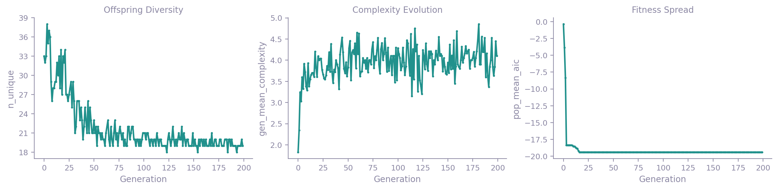
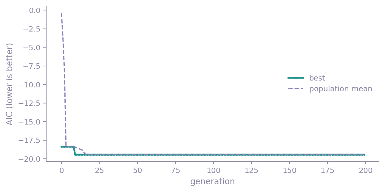
The recorder exposes best_aic, gen_best_aic, gen_best_nmse, gen_mean_aic, gen_mean_complexity, n_valid and n_unique. The gen_* series describe newly evaluated offspring; pop_mean_aic describes the surviving population. A flat best-score curve records a lack of improvement on that run, and does not establish whether the structure is correct.

References

Chen et al. (2022). "Symbolic genetic algorithm for discovering open-form partial differential equations (SGA-PDE)". Phys. Rev. Research 4, 023174. Paper · arXiv:2106.11927

Code: YuntianChen/SGA-PDE

Implementation notes. KD's SGA was ported from an earlier implementation of SGA-PDE. It preserves the paper's three-tree construction at the standard width and STRidge column normalization (normalize=2), with crossover pairing and the two-stage selection order checked against that implementation. Protected division keeps mixed-zero divisors finite. The tree finite-difference implementation uses a five-point fourth-order stencil, with a three-point stencil on shorter arrays, where the reference used three-point second-order differences. Zero or non-finite MSE, and fits with empty support, receive infinite AIC.

Only first-order derivative terminals are precomputed; higher orders come from tree composition. There is no literal-zero terminal or param_fields injection for non-differentiable parameter fields. The term executor and data layer have different boundary stencils, so a precomputed derivative and its tree-composed equivalent can differ at boundaries.

Worked example

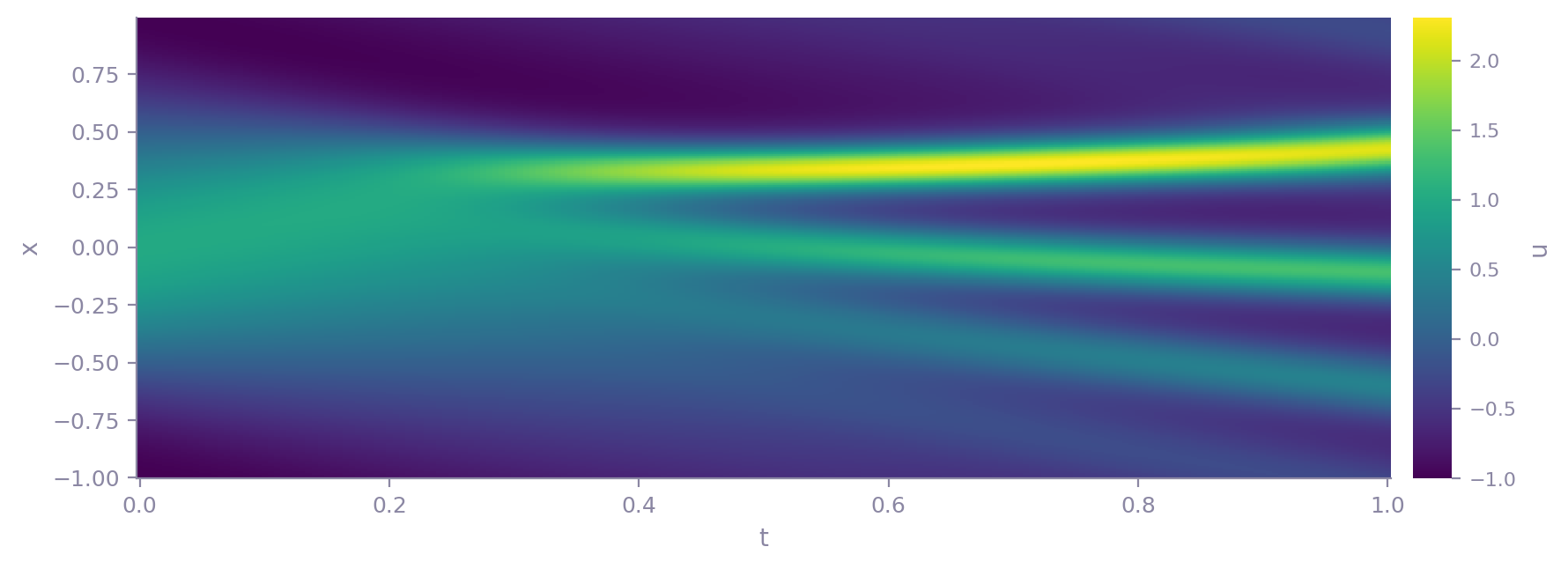
The run below uses the KdV dataset that ships with KD: a 256 × 201 grid whose cosine initial condition steepens under the nonlinear term and then breaks into a train of solitary waves that separate at different speeds, the tallest of them reaching an amplitude of 2.3.

The observed field over its physical spatial and time coordinates.

Running the snippet above, model.best_expr_ is:

SGA-PDE · kdv · seed 42 generation 200 / 200 · nmse 2.70e-06 · AIC -19.42

\(u_t =\)\(-u\,u_x\)\(-0.0025\,u_{xxx}\)

	Equation
Discovered	\(u_t = -u\,u_x -0.0025\,u_{xxx}\)
Reference	\(u_t = -u\,u_x -0.0025\,u_{xxx}\)

Both terms and both coefficients match. The search was not narrowed to them: SGA-PDE was given no candidate library, so the two terms were assembled from operators during the run, and the two coefficients came from its own sparse regression rather than from a fit against the answer.

The fitted derivative target, its equation prediction, and predicted minus measured values. The first two panels share a color scale; the residual has its own scale, with any clipping disclosed on the figure.

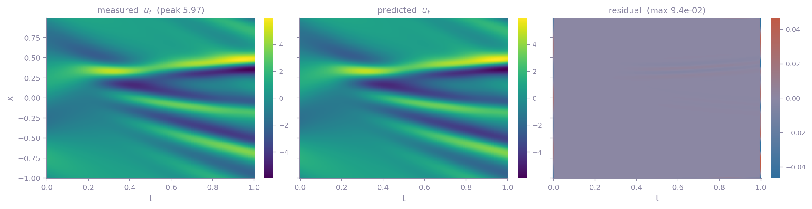
Example diagnostics

The search is recorded as well. kd.VizEngine renders the per-generation record; alongside the universal convergence curve, SGA-PDE contributes diagnostic panels of its own, three of which this run drew (the full list is under Visualization):

The best native score is shown above the algorithm's population diagnostic, when one is recorded. Each panel retains its own score scale.

The algorithm's diagnostic panels, using the same data and plot functions as the full report.

viz = kd.VizEngine(output_dir="out/kdv")
viz.render_all(model.result_, algorithm=model.algorithm_, dataset=dataset)

Full report

Full HTML report from the same run, with all figures, captions and raw result data.