Use your own data
This example builds a dataset from two coordinate arrays and one field array, which is the form most simulation output and most gridded measurements already have. The other examples start from a dataset shipped with KD.
The field below is generated with NumPy to give the example concrete data. Substituting your own arrays requires no other change.
Build the dataset
kd.PDEDataset.from_arrays needs three things: one 1-D array per coordinate
axis, one field array shaped to those axes in order, and the name of the term
that goes on the left-hand side. The full contract is under
Data requirements.
import numpy as np

import kd

k = 0.1
x = np.linspace(0.0, 1.0, 128)
t = np.linspace(0.0, 0.5, 101)
X, T = np.meshgrid(x, t, indexing="ij")
u = np.exp(-(np.pi**2) * k * T) * np.sin(np.pi * X) + 0.5 * np.exp(
    -4 * (np.pi**2) * k * T
) * np.sin(2 * np.pi * X)

dataset = kd.PDEDataset.from_arrays(
    coords={"x": x, "t": t},
    fields={"u": u},
    lhs="u_t",
    name="my-data",
)
kd.preview(dataset)
Dataset: my-data
Axes:
     x | n=128  | range [0.000, 1.000] | step 0.007874 (uniform)
     t | n=101  | range [0.000, 0.500] | step 0.005 (uniform)
Fields:
     u | dtype=float64 | shape=(128, 101) | min=0.000 max=1.299 mean=0.499 (NaN=0)
LHS: u_t  (field='u', axis='t')
Status: ready to fit
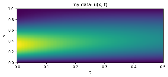
kd.preview reports what KD read: the axes and their spacing, the field and
its range, and the left-hand side it will fit. Status: ready to fit means
the dataset satisfies the contract.
kd.viz.plots.plot_field(dataset)
Fit an algorithm
Fitting is a single call. seed makes the run reproducible, and generations
sets the search budget.
model = kd.Model(algorithm="sga", generations=20, seed=2, verbose=False).fit(dataset)
model
Model(algorithm='sga', fitted=True, best_expr='u_t = 0.09998*u_xx', best_score=-24.38)
The displayed second derivative u_xx identifies the heat equation the field
was built from. Raw term exports spell it diff2_x(u); the same IR vocabulary
is used by every algorithm and is described under
Equation representation.
The displayed score is SGA-PDE AIC; lower values indicate a better fit under that criterion.
Render the report
model.report writes every figure that applies to this fit, plus one HTML
page collecting them. The report is displayed inline below.
model.report("../out/my_data")
Report: ../out/my_data/report.html
Measured data
The derivatives above came from finite differences on the grid, which suits
clean simulation output. For measured data, pass derivatives="autograd" to
kd.Model: KD then fits a smooth surrogate to the field and differentiates
that, which handles noise and points that are not evenly spaced. The two
routes are compared under Derivative sources.
Next steps
- Getting started -- the same workflow on a bundled benchmark, with more of the result surface explained.
- Breaking waves -- a published result reproduced on real wave-tank measurements.
- Algorithms -- what each of the seven searches, and a worked example for each.