DLGA-PDE

A neural network fits the field and supplies derivatives; a genetic algorithm searches term sets over a candidate library.

algorithm

dlga

score

DLGA fitness min

cost

heavy

derivatives

autograd

equation form

EVOLUTION

data layout

grid

Usage

import kd

dataset = kd.load_burgers()
model = kd.Model(algorithm="dlga", generations=40, seed=1, pop_size=40)
model.fit(dataset)

Main parameters

Parameter	Default	Resume	Description
`pop_size`	`400`	resume-safe	Genetic population size.
`epsilon`	`0.001`	resume-safe	Expression-length penalty.
`mutation_rate`	`0.4`	resume-safe	Genome mutation probability.
`crossover_rate`	`0.8`	resume-safe	Genome crossover probability.
`surrogate_lr`	`0.001`	init-only	Neural-surrogate learning rate.

All fields of DLGAConfig

Field	Type	Default
`mode`	`Literal['constant', 'adaptive', 'auto']`	`constant`
`library`	`list[str]`	`['u', 'u_x', 'u_xx', 'u_xxx']`
`solver`	`Literal['svd_null_space', 'ols']`	`svd_null_space`
`lhs_auto_select`	`bool`	`False`
`target_lhs_order`	`int`	`1`
`epsilon`	`float`	`0.001`
`pop_size`	`int`	`400`
`seed`	`int`	`0`
`auto_upgrade_threshold`	`float`	`0.001`
`max_modules`	`int`	`5`
`max_module_length`	`int`	`5`
`partial_prob`	`float`	`0.6`
`genes_prob`	`float`	`0.6`
`crossover_rate`	`float`	`0.8`
`mutation_rate`	`float`	`0.4`
`add_rate`	`float`	`0.4`
`delete_rate`	`float`	`0.5`
`surrogate_hidden_sizes`	`list[int]`	`[50, 50, 50, 50, 50]`
`surrogate_activation`	`Literal['tanh', 'sin', 'relu']`	`sin`
`surrogate_lr`	`float`	`0.001`
`surrogate_max_epochs`	`int`	`50000`
`surrogate_patience`	`int \\| None`	`None`
`surrogate_val_ratio`	`float`	`0.2`
`surrogate_restore_best`	`bool`	`True`

Search space

DLGA-PDE searches sums of products drawn from a candidate library, fitting constant coefficients. Reachable expressions are polynomials in the supplied field and derivative tokens. Use the dataset's own field and axis names: u_x_t is a mixed partial, and diff_t(u_x) is its open-form spelling. An atomic name segment is limited to third order; higher compound derivatives can be written as u_xx_xx.

The library determines which axes can enter a result. A library token that names an unknown field or axis, or a dataset field other than the left-hand-side one, refuses the whole fit before training. So does, when no sketch is set, a token that spells a time derivative of the left-hand-side field that the run fits: the order target_lhs_order names (u_t, diff_t(u), diff1_t(u) for order 1; u_tt, diff2_t(u) for order 2), or both orders while lhs_auto_select is on. Such a token would fit its own branch exactly. The time derivative of an order the run does not fit is an ordinary library token. An atomic segment above third order, such as u_xxxx, is not refused: the fit runs and every candidate containing that token is invalid, so use the u_xx_xx spelling. The surrogate models only the left-hand-side field; other fields and their derivatives cannot enter its library. The constant-coefficient stage is implemented; the adaptive variable-coefficient modes are rejected at construction.

Surrogate fitting precedes genetic search and can dominate cost. Both the number of observations and the derivative library affect resource use; the epoch budget alone does not bound memory. A shorter fit changes derivative accuracy and, under lhs_auto_select, can change the selected left-hand-side order. No pretrained weights or optional backend are needed.

Method

A neural network first fits the observations over their coordinates. The architecture has five hidden layers of 50 units, sin activation and Adam optimization. Field reads and derivatives both come from this network, with derivatives obtained by autograd.

A genome contains up to max_modules modules of up to max_module_length tokens. Each module is a product and the genome is their sum. Coefficients are found from the augmented system's null space or by ordinary least squares, according to solver. Fitness is nmse + epsilon * length, with length counted in tokens. Each candidate is fitted against the time derivative of the order target_lhs_order names, which has to equal the dataset's own left-hand-side order. With lhs_auto_select enabled, each candidate is fitted against both the first and second time derivative and the branch with the lower NMSE is used, so the returned law can carry the order the dataset does not declare.

Each generation scores the population, retains the better half, refills it with random genomes, exchanges a module between adjacent pairs, then mutates by adding or deleting a module and shifting a token to an adjacent library entry. Library order therefore affects mutation. One generation is one KD iteration, controlled by generations.

Result interpretation

model.best_score_ combines the fit error with the per-token length penalty, so NMSE alone does not rank term sets. NMSE is measured against the network's field and derivatives, which are the quantities used during search. model.result_.equation carries the fitted terms, coefficients and selected left-hand side. The returned coefficients come from KD's refit over the selected structure on that surrogate domain.

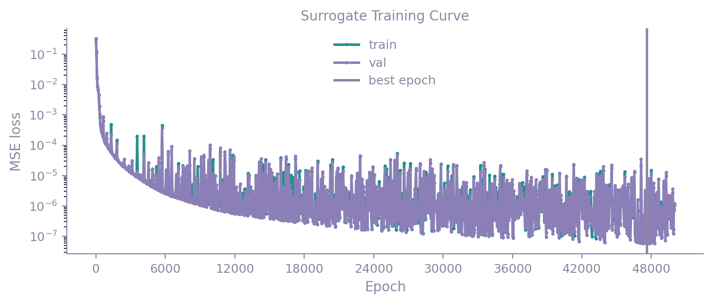
The recorder distinguishes surrogate training from genetic search. Read the training and validation losses alongside the per-generation fitness, diversity and complexity series. A small NMSE is evidence of a fit on that domain, and does not by itself establish recovery of the generating equation. If changing the seed or population budget improves the result, the search budget was relevant; repeated poor fits also warrant checking the library and surrogate accuracy.

References

Xu et al. (2020). "DLGA-PDE: Discovery of PDEs with incomplete candidate library via combination of deep learning and genetic algorithm". J. Comput. Phys. 418, 109584. Paper · arXiv:2001.07305

Code: woshixuhao/DLGA_tutorial (the author's tutorial notebook, on the KdV case), woshixuhao/PIC_code (the author's own code for a later paper, running the same neural-network-plus-genetic-algorithm search)

Implementation notes. The paper treats the order of the time derivative as part of what is discovered: the left-hand side is a gene of the genome, changed by mutation, and genomes with different left-hand sides compete on fitness. By default KD takes the order from the dataset and fits only that left-hand side. An earlier implementation fits u_t and u_tt for every candidate and keeps the better branch, which is lhs_auto_select=true here; under that option KD compares the branches by NMSE. The paper's Eq. (6) and that implementation compare raw MSE, which also varies with the target branch's variance. The length penalty is configurable; the author's tutorial fixes it for its demonstration. The genetic mechanism is checked against that implementation, with corrected crossover indexing and selection of candidates with duplicate fitness values. The adaptive variable-coefficient extension is not part of this implementation.

Worked example

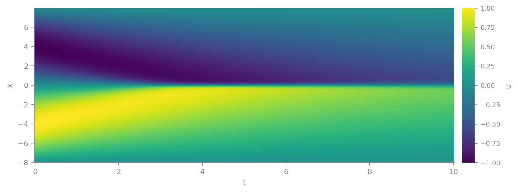
The run below uses the Burgers dataset that ships with KD: a 256 × 201 grid over x in [-8, 8) and t in [0, 10], whose initial profile steepens into a front at the origin and then spreads out as the diffusive term takes over.

Heatmap of the Burgers field u(x, t) — The observed field over its physical spatial and time coordinates.

The equation returned by the run:

	Equation
Discovered	\(u_{t} = - 0.9993 u u_{x} + 0.0999 u_{xx}\)
Reference	\(u_t = -u\,u_x +0.1\,u_{xx}\)

Both terms and both coefficients match. The terms were assembled from the default candidate library (u, u_x, u_xx, u_xxx), and every candidate was fitted against u_t alone under the default target_lhs_order=1 and lhs_auto_select=False. Setting lhs_auto_select=True enables the paper's two-branch selection, fitting each candidate against both u_t and u_tt and keeping the branch with the lower NMSE.

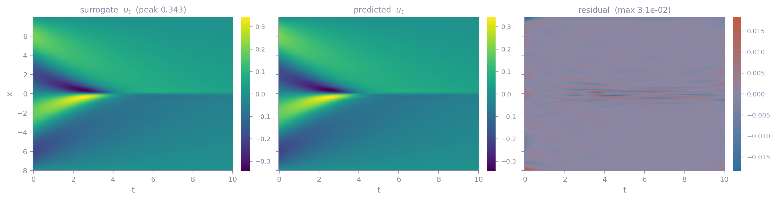
Surrogate u_t, predicted u_t, and the residual between them — The surrogate derivative target, its equation prediction, and predicted minus surrogate values. The first two panels share a color scale; the residual has its own scale, with any clipping disclosed on the figure.

Example diagnostics

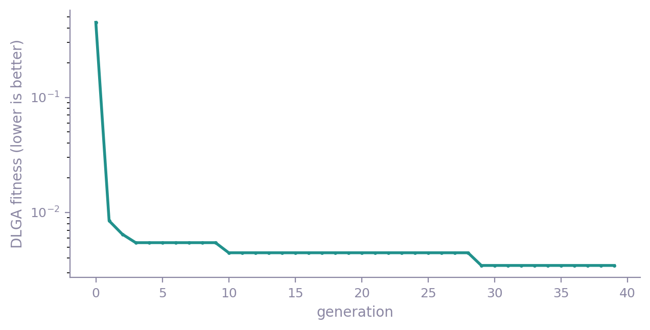
This run has DLGA fitness 0.00346122 and NMSE 0.0004612.

Fitness adds the configured length penalty to NMSE.

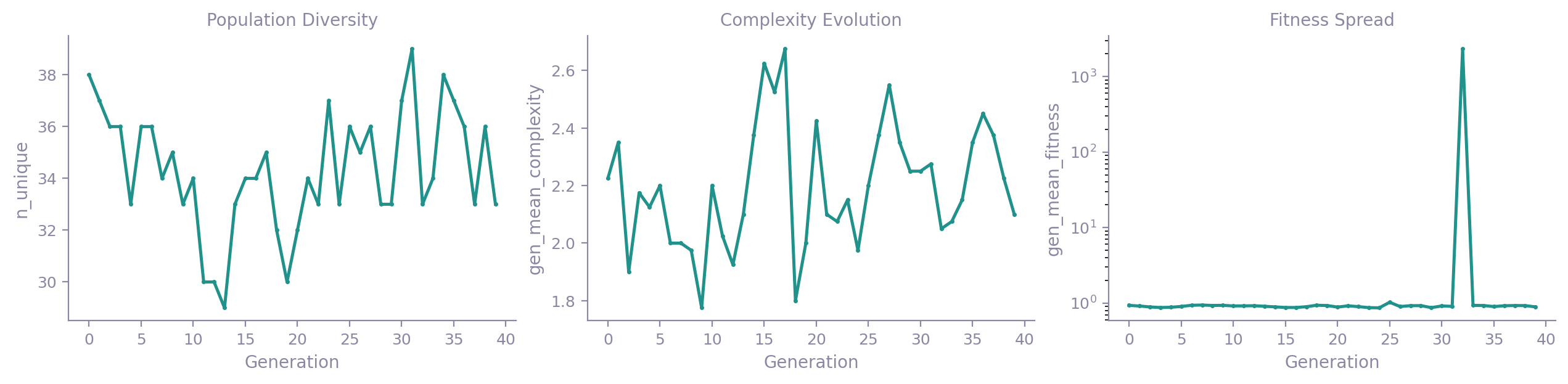
The search is recorded as well. kd.VizEngine renders the per-generation record; alongside the universal convergence curve, DLGA-PDE contributes four diagnostic panels of its own (the full list is under Visualization):

Best DLGA fitness per generation — The best native score recorded by the search. The axis label identifies the score and its direction.

Population diversity, complexity evolution and fitness spread panels — The algorithm's diagnostic panels, using the same data and plot functions as the full report.

The fourth panel shows the training of the surrogate network, which is independent of the search:

Training and validation loss of the neural surrogate per epoch — Training and validation loss of the surrogate; the marked epoch identifies the retained weights.

viz = kd.VizEngine(output_dir="out/burgers")
viz.render_all(model.result_, algorithm=model.algorithm_, dataset=dataset)

Full report

Full HTML report from the same run, with all figures, captions and raw result data.