Noisy Burgers walkthrough: a field with 15% noise, and its equation
KD recovers the Burgers equation, u_t = -u u_x + 0.1 u_xx, from the bundled
benchmark field after 15% relative Gaussian noise is added to every sample. The
search is DLGA, which first fits a neural network to the noisy field and takes
every derivative from that network instead of from the samples; Xu et al. (2020)
report Burgers recovered at this noise level, and KD's recovery suite pins the
same case. Four calls carry the walkthrough: load and noise the data, draw it,
fit, render the report. Every output below is committed from one execution.
import kd
The data
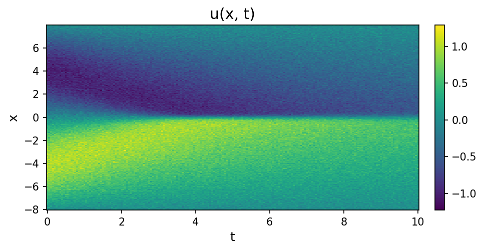
kd.load_burgers ships the 256 by 201 Burgers field of the SGA-PDE benchmark
set. kd.add_noise returns a copy with Gaussian noise whose standard deviation
is 15% of the field's own; the seed fixes the draw, and noise_level on the
result records what was added. kd.preview audits the grid and the field,
plot_field draws it as it would be measured.
dataset = kd.add_noise(kd.load_burgers(), 0.15, seed=2026)
kd.preview(dataset)
Dataset: burgers
Axes:
     x | n=256  | range [-8.000, 7.938] | step 0.0625 (uniform)
     t | n=201  | range [0.000, 10.000] | step 0.05 (uniform)
Fields:
     u | dtype=float64 | shape=(256, 201) | min=-1.226 max=1.288 mean=0.000 (NaN=0)
LHS: u_t  (field='u', axis='t')
Status: ready to fit
kd.viz.plots.plot_field(dataset)
Differentiate the samples directly
Finite differences of a noisy field amplify the noise: at this level the
derivative columns carry little of the signal, and a search over them keeps
whatever fits the noise. SGA-PDE at the budget its Burgers recovery suite
validates on the clean field (100 generations, seed 42) returns
u_t = 0.002134 u^2 x^3 here, a term with no derivative in it, after about
3 minutes.
direct = kd.Model(algorithm="sga", generations=100, seed=42, verbose=False).fit(dataset)
print(f"Discovered : {direct.result_.equation}")
print(f"Reference  : {dataset.ground_truth}")
Discovered : u_t = 0.002134*u**2*x**3
Reference  : u_t = -u * u_x + 0.1 * u_xx
Fit DLGA
DLGA fits a neural network to the noisy samples and takes every derivative,
u_t included, from that network. DLGAConfig.burgers_preset locks the
length penalty validated for Burgers; surrogate_max_epochs=50_000 is the
network's training budget, and pop_size=50 with generations=20 is the
genetic search budget the recovery suite runs at. The fit took about 158
minutes in this run.
model = kd.Model(
    algorithm="dlga",
    generations=20,
    config=kd.DLGAConfig.burgers_preset(pop_size=50, seed=0, surrogate_max_epochs=50_000),
    verbose=False,
).fit(dataset)
model
DLGA recovered expression has nmse=0.0258 and length=8 tokens. The default epsilon=1e-03 was tuned for raw-MSE-era fitness magnitudes; under the NMSE-era selector the length penalty contribution is smaller, so the GA may include small-coefficient noise terms. Truth structure is still recovered (see is_recovery_success superset match). To get a cleaner surface expression, raise DLGAConfig.epsilon to ~1e-2 to 5e-2 — see DLGAPlugin docstring for per-PDE recommendations.


Model(algorithm='dlga', fitted=True, best_expr='u_t = -0.9829*u*u_x - 0.002841*u*u_xxx + 1.184e-6*u_x*u_xxx**2 + 0.1039*u_xx', best_score=0.03381)
Recovered law and the reference
DLGA prints the structure it selected; the fitted coefficients are on the
equation panel of the report below. In this run they are -0.9829 for
u u_x (reference -1, relative error 1.7%) and 0.1039 for u_xx
(reference 0.1, relative error 3.9%). Two further terms stayed in the
expression with coefficients far below those two, -0.002841 u u_xxx and
1.184e-6 u_x u_xxx^2; the fit's NMSE is 0.0258. The warning printed by the
fit says the same thing about them: at epsilon=1e-3 the length penalty
leaves such small-coefficient terms in, and a larger epsilon shortens the
expression.
print(f"Discovered : {model.result_.equation}")
print(f"Reference  : {dataset.ground_truth}")
Discovered : u_t = -0.9829*u*u_x - 0.002841*u*u_xxx + 1.184e-6*u_x*u_xxx**2 + 0.1039*u_xx
Reference  : u_t = -u * u_x + 0.1 * u_xx
The report
model.report renders every figure this fit supports and one HTML page that
embeds them: the convergence curve, the parity plot, the equation and its
tree, the coefficient bars, the residual figures, the noisy field next to the
field integrated from the discovered equation, the time slices, the error
heatmap, the PDE residual field, and DLGA's own diagnostics, including the
training curve of the network that supplied the derivatives. The page is
shown below; the same files are written to the output directory.
model.report("../out/noisy_burgers_walkthrough")
Report: ../out/noisy_burgers_walkthrough/report.html
Next steps
kdv_walkthrough.ipynb: the same four calls on a clean field, with SGA-PDE differentiating the samples directly.08_dlga.py: DLGA on a synthetic Burgers field at a small budget, as a script.09_compare_algorithms.py: every algorithm on one dataset, scored with one ruler.